Learning ML
I’ve decided to embark on the journey of mastering machine learning. I have my own personal goals to build systems that can think and learn on it’s own. As a step to getting closer to this goal I’ve decided to take the Machine Learning Specialization course by Andrew Ng.
Suffice to say the course is of top notch quality, and I highly recommend it to anyone who wants to truly understand what’s happening behind the scenes rather than just using existing llms / rags and reading stuff over the internet. It will open you up to a whole new world with a deep level of understanding of the math and the science behind how ‘AI’ actually works.
Method to the Madness
I love working with Elixir programming language and it’s ecosystem. I’ve built various tools, apps and companies in Elixir and want to be able to use Elixir for my machine learning work. Suffice to say Elixir is where I excel when it comes to building things. The tooling around Elixir’s machine learning ecosystem has improved significantly over the past months and I’ve decided to use it as the primary way to apply all the lab work that is in the course I mentioned above.
Given that the course provides code written in python I would have to translate the code an apply my learnings using the tooling around elixir. This is a great way to learn my way around all the tooling available in Elixir’s ML portfolio. The course provides jupyter notebook with outputs I used to validate my code in elixir is returning the same values.
Once I get a good grip with what’s provided in the course, I would also go back and try examples in the Machine Learning in Elixir book. This whole process has been extremely productive and I’ve been very happy with the outcome.
Challenge Accepted
I won’t lie and say that my method to learning is perfect and smooth. I’ve lost days (and hair, at this point there isn’t much left 🤣) trying to figure out why something isn’t working, only to realize later it wasn’t my code, but a bug in the tooling. It certainly has it’s challenges, however it also taught me a lot. Within the span of 3 weeks I’ve learned what all the tools do and how to use them. While I don’t claim to be an expert in anyway, it has at the very least help me learned the full flow and all the components involved. I’m starting to see ways of architecting my own models for doing some things I’ve been pondering on for a while. Given all the challenges I’ve faced and I’m sure there are more to come, I wouldn’t do things any differently. I love Elixir, and my mind just works better when I’m in Elixir land.
Let’s start by taking a look at some of the tooling.
Livebook
In the python ecosystem there are 2 primary notebooks, google’s colab which is a hosted notebook and comes with GPU out of the box, and jupyter notebook / jupyter labs which you can run locally on your own computer.
In Elixir livebook is the defacto standard, and has an amazing user experience. I love working with livebook.
Nx
This is the library for working with numerical data. In machine learning everything is expressed as mathematical expressions and numbers. Nx is the library that will allow you to do this. It is the equivalent to Numpy in Python. Let’s take a look at some code.
Mix.install([
  {:nx, "~> 0.7"},
  {:exla, "~> 0.7"}
])

Nx.global_default_backend(EXLA.Backend)

# change the client as you see fit.
Nx.Defn.default_options(compiler: EXLA, client: :cuda)
Creating a tensor
# python
X = np.array([[200., 100.]])
# elixir
x = Nx.tensor([[200, 100]])Returning the shape
# python
X.shape
# elixir
Nx.shape(x)Mathematical expression
# python
w = np.array([10])
b = 5

f_x = np.dot(w, X) + b
# elixir
w = Nx.tensor([10])
b = 5
f_x =
Nx.dot(w, x)
|> Nx.add(b)With Elixir if you wish to use normal mathematical expression you can also use Nx.Defn
defmodule LinearAlgebra do
  import Nx.Defn

  defn run(x, w, b) do
    Nx.dot(w, x) + b
  end
end

f_x = LinearAlgebra.run(x, w, b)
Notice I’m not using a standard def to define the function but defn. This allows me to express mathematical expression much closer to how it’s often expressed in mathematics. It also has the added benefit of being JIT compiled.
Looping
# python
m = X.shape[0]

cost_sum = 0

for i in range(m):
    f_wb = w * x[i] + b
    cost = (f_wb - y[i]) ** 2
    cost_sum = cost_sum + cost

total_cost = cost_sum / (2 * m)

return total_cost
# elixir
defmodule LinearRegression do
import Nx.Defn
defn compute_cost(x, y, w, b) do
{m, _} = Nx.shape(x)
cost = Nx.tensor(0.0, type: :f64)
range = 0..(m - 1)
{cost_sum, _, _, _, _} =
while {cost, x, y, w, b}, i <- range, unroll: true do
f_wb_i = Nx.dot(x[i], w) + b
{cost + (f_wb_i - y[i]) ** 2, x, y, w, b}
end
cost_sum / (2 * m)
end
endIn elixir you can use for loops and Enum.reduce as well. However if you want to live in defn land an experience all the benefits of JIT compilation you’ll have to use the while loop from elixir’s Nx library. You can also get extra benefit by adding unroll: true. It will actually unroll your while loop as if you wrote out every iteration by hand. Be careful with unroll though, if you have a lot of iterations in your range like 10,000 using unroll: true can be a disaster 🧨😅. Using something like unroll: 2 would be more wise.
Axon
When building neural networks we will need to leverage Axon. In python the equivalent is tensorflow, pytorch and jax. The python ecosystem also has keras which sits on top of tensorflow, pytorch or jax. It makes building neural networks simple by providing some higher level of abstractions.
A word about axon version. As of writing this the latest published version of axon is 0.6.1 it has some flaws when training models. It simply doesn’t work correctly. I recommend using github: ‘elixir-nx/axon’ in your mix file.
Mix.install([
  {:axon, github: "elixir-nx/axon"}
])
Let’s take a look at the differences.
Model Creation
# python
model = Sequential(
  [
    tf.keras.Input(shape=(2,)),
    Dense(3, activation='sigmoid', name = 'layer1'),
    Dense(1, activation='sigmoid', name = 'layer2')
  ]
)
# elixir
model =
Axon.input("input", shape: {nil, 2})
|> Axon.dense(3, activation: :sigmoid, name: "layer1")
|> Axon.dense(1, activation: :sigmoid, name: "layer2")You’ll notice they look almost the same. Axon provides really nice API for building models out of the box.
Inspecting the Model
# python
model.summary()
Model: "sequential_2"
_________________________________________________________________
Layer (type) Output Shape Param #
=================================================================
layer1 (Dense) (None, 3) 9
layer2 (Dense) (None, 1) 4
=================================================================
Total params: 13
Trainable params: 13
Non-trainable params: 0
_________________________________________________________________For Axon to be able to output a table below, you’ll need to make sure you have :table_rex library in your mix file.
# elixir
Axon.Display.as_table(model, Nx.template({2, 2}, :f32))
|> IO.puts()
+----------------------------------------------------------------------------------------------------+
| Model |
+=================================+=============+==============+=================+===================+
| Layer | Input Shape | Output Shape | Options | Parameters |
+=================================+=============+==============+=================+===================+
| input ( input ) | [] | {2, 2} | shape: {nil, 2} | |
| | | | optional: false | |
+---------------------------------+-------------+--------------+-----------------+-------------------+
| layer1 ( dense["input"] ) | [{2, 2}] | {2, 3} | | kernel: f32[2][3] |
| | | | | bias: f32[3] |
+---------------------------------+-------------+--------------+-----------------+-------------------+
| sigmoid_0 ( sigmoid["layer1"] ) | [{2, 3}] | {2, 3} | | |
+---------------------------------+-------------+--------------+-----------------+-------------------+
| layer2 ( dense["sigmoid_0"] ) | [{2, 3}] | {2, 1} | | kernel: f32[3][1] |
| | | | | bias: f32[1] |
+---------------------------------+-------------+--------------+-----------------+-------------------+
| sigmoid_1 ( sigmoid["layer2"] ) | [{2, 1}] | {2, 1} | | |
+---------------------------------+-------------+--------------+-----------------+-------------------+
Total Parameters: 13
Total Parameters Memory: 52 bytesElixir can also output the model graph:
Axon.Display.as_graph(model, Nx.template({2, 2}, :f32))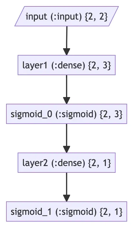
Data Preparation
In elixir’s ecosystem there are 2 libraries that will help you with data preparation and simplifying some operations. They are :scholar and :explorer.
Explorer is useful for loading and manipulating data it leverages polars library written in rust, so your data manipulation and exploration is fast. Explorer will also allow you to load data from various types of files such as csv, parquet, ndjson and Apache Arrow IPC.
Shcolar is more of a toolkit that contains implementations that are ready to use out of the box.
Both these tools work natively with Nx which means they complement each other beautifully.
Normalization
When training neural networks normalizing your data can help with speeding up the training process. It helps with the gradient descent process.
The below example will normalize the data and use 0,0 on the axis as the center, so the output of the normalized values will be between -x, and x. It simply takes the value - mean(value) / standard_deviation(value)
# python
norm_l = tf.keras.layers.Normalization(axis=-1)
norm_l.adapt(X)
Xn = norm_l(X)
Notice the norm_l.adapt(X) it will basically calculate the mean and the standard deviation of a given dataset. This will be important later when you do inference with the model.
X is the dataset containing values like this [[200, 12], [230, 18]]
In elixir you can normalize your data in various ways. You can use the :explorer library or :scholar. I however prefer :scholar for reasons I’ll mention soon.
# with explorer

require Explorer.DataFrame, as: DF

df = DF.new(%{
  x1: [200, 230],
  x2: [12, 18]
})

normalized =
  DF.mutate(
    df,
    for col <- across(["x1", "x2"]) do
      {col.name, (col - mean(col)) / standard_deviation(col)}
    end
  )
The problem with the above approach is it’s quite verbose and also it’s stateless which means if you want to get the mean and standard_deviation of a particular dataset you’ll have to write that part as well. But it does give you the power to implement any kind of normalization technique you want.
If you just want to normalize based on the standard methods, then I recommend using scholar.
# with scholar

require Explorer.DataFrame, as: DF

df = DF.new(%{
  x1: [200, 230],
  x2: [12, 18]
})

dataset =
  Nx.stack(df[["x1", "x2"]], axis: -1)

scaler = Scholar.Preprocessing.StandardScaler.fit(dataset)

normalized = Scholar.Preprocessing.StandardScaler.transform(scaler, dataset)
What I want to highlight here is the fit part generates the mean and standard_deviation for you based on the dataset you pass in. This will be necessary when you do inference after training the model. It’s important to store this state somewhere. With scholar you can also simply use Scholar.Preprocessing.StandardScaler.fit_transform(dataset) if you are sure you won’t need the scaler.
Model Training
This is the “learning” part of machine learning. In python you can simply pass your Xt the x training data and Yt y training data. Where x is the actual data and y in this case is the labels.
# python
model.compile(
  loss = tf.keras.losses.BinaryCrossentropy(),
  optimizer = tf.keras.optimizers.Adam(learning_rate=0.01),
)

model.fit(Xt, Yt, epochs=10)
With keras you can simply pass the training data and labels in without batching. Internally by default keras handles batching for you already. It uses a batch size 32 by default.
With Elixir we will do that with Nx.
# elixir
train_data = Stream.zip(Nx.to_batched(normalized, 32), Nx.to_batched(y_train, 32))

state = Axon.ModelState.new(%{})

optimizer = Polaris.Optimizers.adam(learning_rate: 0.01)

trained_state =
  model
  |> Axon.Loop.trainer(:binary_cross_entropy, optimizer)
  |> Axon.Loop.metric(:accuracy)
  |> Axon.Loop.run(train_data, state, epochs: 10)
The above code will use the :binary_cross_entropy as the loss function. You can also construct your own loss function if you wish.
Inference
Now that we’ve trained our model let’s see the difference in inference.
# python
input = np.array([
    [200,12.2],
    [150,17]
  ])
input_normalized = norm_l(input)
predictions = model.predict(input_normalized)
Notice how we have to normalize the input before passing it into the predict function. This is why having a stateful normalization is important. We’ll see how this is done in elixir.
# elixir
input = Nx.tensor([[200, 12.2], [150, 17]])

input_normalized =
  Scholar.Preprocessing.StandardScaler.transform(scaler, input)

prediction = Axon.predict(model, trained_state, input_normalized)
You’ll notice that for our normalization we call transform and pass it the scaler that was generated from the training data set. This will ensure our prediction is correct.
Note that for experimentation using Axon.predict/3 is enough. However for production it is recommended to use Nx.Serving see more on that in the documentation.
Closing Thoughts
I hope that this post will help some people who are trying to get into machine learning with Elixir. There is a lot more to share than what’s presented in this post. There is a whole topic with data visualization with :vega_lite and kino which I didn’t touch on. I think those libraries deserve their own post, and I do plan on covering it in a future post. If you enjoyed this post do give me an upvote, like and a retweet.
If I made any mistakes I apologize in advance. Do feel free to reach out and let me know.